Heat advection and diffusion¶

General equation¶

If we add advection and internal heat generation to our heat equation, we get

\begin{equation} \rho C_p \left(\frac{\partial T}{\partial t} + v_x\frac{\partial T}{\partial x}\right) = k \frac{\partial^2 T}{\partial x^2} + H \end{equation}

If we rearrange the terms to have only the time derivative on the left-hand side, we get

\begin{equation} \frac{\partial T}{\partial t} = \frac{k}{\rho C_p} \frac{\partial^2 T}{\partial x^2} + \frac{H}{\rho C_p} - v_x\frac{\partial T}{\partial x} \end{equation}

Exercise - Advection and diffusion¶

Write the finite difference approximation (i.e., discretize) the advection-diffusion equation. Use the forward difference in time and the central difference in space. Write the expression in form

\begin{equation} T_i^{q+1} = \ldots~T^q~\mathrm{terms~only~on~this~side}~\ldots \end{equation}
Modify the intrusion code below (or use the one you modified previously):
- Add variables that store the internal heat production \(H\) and the advection velocity \(v_x\) (what are suitable values?)
- Modify the line within the time loop that calculates the next value of \(T\): include the terms for heat generation and advection
Start with \(H=0\) and \(v_x = 0\). Gradually change these values.
- How do the results change as you give non-zero values for these terms?
- What happens if \(v_x > 0\) compared to \(v_x < 0\)?
- What if \(v_x\) has a large (positive or negative) value?

Extra tasks¶

Remove the initial hot intrusion. Instead, add spatially variable internal heat generation. For this, you will need to introduce new numpy array (of size nx), fill it with values of internal heat generation, and use it (H[ix] instead of H) when you calculate the new temperature value.
Calculating the heat flow
- Heat flow is defined as \(q=k\frac{dT}{dx}\). Write an approximation for \(q\) by replacing the derivative with a finite difference expression.
- Modify the code so that you create an array (of size nt) that stores surface heat flow values each time step. Within the time loop, calculate each time step the heat flow between two topmost grid points.
- After the time loop, plot the recorded surface heat flow history.

import numpy as np
import matplotlib.pyplot as plt

yr2sec = 60*60*24*365.25  # num of seconds in a year

# Set material properties
rho = 2900   # kg m^-3
Cp = 900     # J kg^-1 K^-1
k = 2.5      # W m^-1 K^-1

# Set geometry and dimensions
L = 35e3         # m
nx = 30          # -
dx = L / (nx-1)  # m
print("dx is", dx, "m")

silltop = 5e3    # m
sillbott = 10e3  # m

# Set total time and time step
t_total = 0.1e6 * yr2sec          # s
dt = 1e4 * yr2sec                 # s
nt = int(np.floor(t_total / dt))  # -
print("Calculating", nt, "time steps")

# Set boundary temperature values and intrusion temperature
Tsurf = 0.0        # deg C
Tmoho = 600.0      # deg C
Tintrusion = 700.0 # deg C

# Create arrays to hold temperature fields
Tnew = np.zeros(nx)
Tprev = np.zeros(nx)

# Create coordinates of the grid points
x = np.linspace(0, L, nx)

# Generate initial temperature field
for ix in range(nx):
    if (x[ix] < sillbott) and (x[ix] > silltop):
        Tprev[ix] = Tintrusion
    else:
        Tprev[ix] = x[ix] * (Tmoho - Tsurf) / L

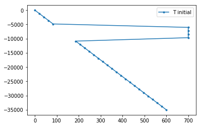
# Plot initial temperature field
plt.plot(Tprev, -x, '.-', label='T initial')
plt.legend()
plt.show()

# Start the loop over time steps
curtime = 0
while curtime < t_total:
    curtime = curtime + dt
    
    # boundary conditions
    Tnew[0] = Tsurf
    Tnew[nx-1] = Tmoho
    
    # internal grid points
    for ix in range(1, nx-1):
        Tnew[ix] = (k * (Tprev[ix-1] - 2.0*Tprev[ix] + Tprev[ix+1]) / dx**2) * dt / (rho * Cp) + Tprev[ix]
        
    # copy Tnew to Tprev
    Tprev[:] = Tnew[:]
    

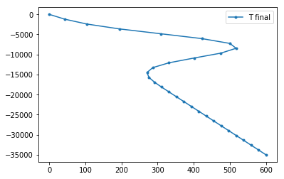
# Plot the final temperature field
plt.plot(Tnew, -x, '.-', label='T final')
plt.legend()
plt.show()

dx is 1206.896551724138 m
Calculating 10 time steps