Finite differences method introduction

The method of finite differences is used, as the name suggests, to transform infinitesimally small differences of variables in differential equations to small but finite differences, thus enabling solution of these equations by means of numerical calculations in a computer.

The starting point for the finite differences method is the definition of a derivative:

\[\frac{\mathrm{d}f}{\mathrm{d}x}\rvert_{x=x_0} = \lim_{\Delta x \rightarrow 0} \frac{f(x_0 + \Delta x) - f(x_0)}{\Delta x} .\]

However, computers can only handle numbers of finite value, not infinitesimally small values such as \(\Delta x\) at the limit used in the definition. Thus, the derivative is approximated by dropping out the limit:

(1)\[\frac{\mathrm{d}f}{\mathrm{d}x}\rvert_{x=x_0} \approx \frac{f(x_0 + \Delta x) - f(x_0)}{\Delta x} .\]

where \(\Delta x\) is sufficiently small. If we could choose arbitrary small values of \(\Delta x\), we would reach the exact value of the derivative, but in reality we are always limited by the numerical accuracy of the computers. [1]

Approximation (1) is called a forward difference. Its counter-part, the backward difference approximation is defined similarly:

(2)\[\frac{\mathrm{d}f}{\mathrm{d}x}\rvert_{x=x_0} \approx \frac{ f(x_0) - f(x_0 - \Delta x)}{\Delta x} .\]

Finally, one can define so called central difference approximation:

(3)\[\frac{\mathrm{d}f}{\mathrm{d}x}\rvert_{x=x_0} \approx \frac{ f(x_0 + 0.5\Delta x) - f(x_0 - 0.5\Delta x)}{\Delta x} = \frac{ f(x_½) - f(x_{-½})}{x_½ - x_{-½}}\]

where \(x_½ - x_{-½} = \Delta x\).

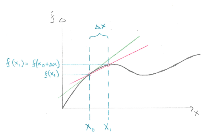
Fig. 1 Illustration of finite differences approximation (forward difference). As \(x_1\) approaches \(x_0\) the approximated gradient (red) approaches the exact gradient of the function \(f_0\) at \(x=x_0\).

Exercise

Sketch a visualization of backward and central differences like the forward differences is visualized in Fig Fig. 1.

Equation (3) can be generalized as

(4)\[\frac{\mathrm{d}f}{\mathrm{d}x}\rvert_{x=x_i} \approx \frac{ f(x_{i+½}) - f(x_{i-½})}{x_{i+½} - x_{i-½}}\]

Where \(i\) is an integer. In other words, the indices can be added or subtracted with any number and the approximation still holds, as long as the addition/subtraction is done on each index in the equation.

Exercise

Write a central difference approximation for \(\frac{\mathrm{d}f}{\mathrm{d}x}|_{x=x_{15}}\)

The central difference approximation can also be written as

\[\frac{\mathrm{d}f}{\mathrm{d}x}\rvert_{x=x_i} \approx \frac{ f(x_{i+1}) - f(x_{i-1})}{x_{i+1} - x_{i-1}}\]

and although generally producing a different value than (4) is still a valid approximation.

The points \(x_1, x_2, x_3, ...\) at which the function \(f\) is evaluated and the derivative approximated, are called grid points. The locations of the grid points are chosen differently depending on the problem one is solving, but they must be in order, so that for all pairs of \(j\) and \(k\), if \(j > k\) then \(x_j > x_k\) (decreasing order is also possible but not usually used). These are the points at which the final solution to the problem (i.e. value of \(f\) in the case above) is to be found.

Often, a regular grid is used. In this case \(\Delta x = x_{i+1} - x_i\) for all \(i\), i.e. the distance between two consequent grid points is always the same.

Conventionally, grid points have indices of integers (0, 1, 2, 3, etc.). Half-indices, like above, may be used in process of deriving the finite differences equation and often required in case of higher order derivatives and/or when using so called staggered grids (see later). The value of a variable in-between two grid points can be found by taking averages, for example

(5)\[x_{i+½} = \frac{x_i + x_{i+1}}{2} ,\]

i.e. assuming linear interpolation between grid points.

Simple example: Throwing a ball

Imagine a man throwing a ball. Let us neglect the resistance by the air and concentrate on the vertical velocity and location of the ball only. The ball leaves the man’s hand at velocity \(V_0\) with vertical component \(V_{z,0}\) at moment \(t=t_0\).

How long will the ball stay in the air?

We know that the vertical velocity of the ball will start to decrease and then turn downwards due to the gravitation. Thus, the velocity of the ball at any given time \(t\) after the throw is \(V_z(t) = V_{z,0} - ½gt^2\).

The simple equation describing the derivative of the vertical location of the ball (i.e. its vertical speed) is

\[\frac{\mathrm{d}z}{\mathrm{d}t} = V_{z,0} - ½gt^2\]

we can discretize this equation using forward difference (1) and thus get

\[\frac{z_{i+1} - z_i}{t_{i+1} - t_i} = V_{z,0} - ½gt_i^2 .\]

Note that also the time on the right hand side now refers to a time at some grid point \(i\). We can rearrange the equation to

\[z_{i+1} = (V_{z,0} - ½gt_i^2) (t_{i+1} - t_i) + z_i\]

which shows that if we know the location of the ball (\(z_i\)) at moment \(t_i\), we can calculate its next position \(z_{i+1}\) at time \(t_{i+1}\), after \(\Delta t\) seconds.

Let’s assume the ball leaves the player’s hand at \(z_0 = 1.8~\mathrm{m}\) at vertical velocity \(V_{z,0} = 15~\mathrm{ms^{-1}}\). Let’s first calculate what is the ball’s elevation after 3 seconds.

We will first choose to divide the time into time steps (i.e. grid spacing) of 0.5 seconds, which will lead to seven grid points.

t (s)	z (m)	i
0.0	1.8	0
0.5		1
1.0		2
1.5		3
2.0		4
2.5		5
3.0		6

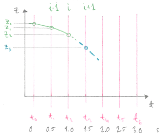
Fig. 2 Illustration of the grid used in the finite differences solution of man throwing a ball. Since the variable here is time, each grid point can also be called a time step.

It is important to keep in mind that the grid index (\(i\)), which is an order number, is separate from the physical values, such as \(t_i\) or \(z_i\). We already know the time and location at time step zero, so we can calculate the location at next time step

\[\begin{split}z_1 &= (V_{z,0} - ½gt_0^2) (t_1 - t_0) + z_0 \\ &= (15 - ½ g \times 0.0^2) (0.5) + 1.8 \\ &= 9.3\end{split}\]

After we know \(z_1\), we can go continue and calculate \(z_2\)

\[\begin{split}z_2 &= (V_{z,0} - ½gt_1^2) (t_2 - t_1) + z_1 \\ &= (15 - ½ g \times 0.5^2) (0.5) + 9.3 \\ &= 16.19\end{split}\]

and so on, until we reach \(z_6\):

t (s)	z (m)	i
0.0	1.8	0
0.5	9.3	1
1.0	16.19	2
1.5	21.23	3
2.0	23.22	4
2.5	20.91	5
3.0	13.08	6

Exercise

Why bother doing the calculations in six steps? Why not take only one step with time step \(\Delta t = 3\mathrm{~s}\)? What would the result be? How does it compare to the six-step solution?

Following is a small Python code snippet that can be used to calculate the ball’s elevation like we just did. You can adjust the starting elevation, the initial velocity, the number of steps to calculate and the total time to calculate.

z = 1.8     # Starting elevation
Vz = 15     # Initial vertical velocity
nt = 6      # In how many steps we do the calculation
tottime = 3 # Total time (s) to calculate
            # The total time and the number of time steps
	    # together implicitly set the size of the time step, dt.

dt = tottime / nt
print ("Size of one time step is:", dt, "seconds")

print ("Time, elevation:")
for it in range(nt):
   t = it * dt
   z = (Vz - 0.5 * 9.81 * t**2) * dt + z
   print(t+dt, z)

Exercise

Experiment with the code snippet: Vary the four parameters and see what is the effect of large or small number of steps taken. Can you estimate how long does it take for the ball to return back to the ground, by varying the number of steps and total time?

How would you try to estimate the exact time it takes for the ball to reach the ground using the python script only? That is, how would you estimate the error of the numerical solution?

Less simple example: Falling sphere in a fluid

In the following, we will use finite differences to solve a simple ordinary differential equation that describes how a solid ball falls down within a viscous fluid.

Stokes’ law relates the frictional resistance of a solid falling sphere in a viscous fluid to the velocity of the sphere:

\[F_D = -6 \pi \eta R v\]

where \(F_D\) is the frictional force, \(\eta\) viscosity of the surrounding fluid, \(R\) radius of the sphere, and \(v\) velocity of the sphere. This force is directed opposite to the direction of the velocity (thus the minus sign). The Stokes’ law is valid at low Reynolds number values [2].

Additionally, we know the gravitational force experienced by the sphere:

\[F_g = -m g ,\]

and the buoyancy force as a function of density of the fluid, \(\rho_f\):

\[F_b = \frac{4}{3}\pi R^3 \rho_f g .\]

Here, \(m\) is the mass of the sphere, and \(g\) acceleration of gravity (\(F_g\) is negative since we have set our z axis to point upwards). The sum of forces experienced by the sphere is thus \(F_s = F_b + F_g + F_D\), and noting that \(F_s = m a_s\) we arrive at

(6)\[m \frac{\mathrm{d}^2 z}{\mathrm{d} t^2} = F_b + F_g - 6 \pi \eta R \frac{\mathrm{d} z}{\mathrm{d} t}\]

where \(z\) is the position (height) of the sphere, and \(t\) time. This differential equation has an analytical solution [3], but we will use finite differences method to solve the equation.

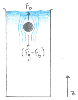
Fig. 3 The fall of the sphere within a viscous fluid is driven by the gravity (\(F_g\)) and resisted by the buoyancy (\(F_b\)) and frictional (\(F_D\)) forces.

Applying finite differences

The derivatives of \(z\) in equation (6) can be approximated using finite differences:

(7)\[\frac{\mathrm{d} z}{\mathrm{d} t}|_{t=t_i} \approx \frac{z_{i+½} - z_{i-½}}{t_{i+½} - t_{i-½}}\]

where \(t_{i-½}\) and \(t_{i+½}\) are two moments in time, so that \(\Delta t = t_{i+½} - t_{i-½}\) is small. Here we have evaluated the derivative (or its approximation) at mid-point between \(t_{i+½}\) and \(t_{i-½}\). Why we have chosen to use “half-steps” instead of full steps \(i \pm 1\) becomes apparent soon.

The second order derivative can be approximated by applying the same rule twice. First,

\[\frac{\mathrm{d}^2 z}{\mathrm{d} t^2}|_{t=t_i} \approx \frac{ \frac{\mathrm{d} z}{\mathrm{d} t}|_{t=t_{i+½}} - \frac{\mathrm{d} z}{\mathrm{d} t}|_{t=t_{i-½}} }{ t_{i+½} - t_{i-½} } .\]

Then the same rule (7) is applied to the first order derivatives within this quotient:

(8)\[\frac{\mathrm{d}^2 z}{\mathrm{d} t^2}|_{t=t_i} \approx \frac{ \frac{z_{i+1} - z_i}{t_{i+1} - t_i} - \frac{z_i - z_{i-1}}{t_i - t_{i-1}} }{ t_{i+½} - t_{i-½} }\]

Note that the first order derivatives in the dividend are evaluated between the the grid points, at \(i+½\) and \(i-½\), which is why the time values in the divisor are chosen at “half-steps”, as well (so that their mid-point is at grid point \(i\) exactly). Assuming a regular grid (\(t_{i+1} - t_i = t_i - t_{i-1} = t_{i+½} - t_{i-½} = \Delta t\)) we get, after simplification,

(9)\[\frac{\mathrm{d}^2 z}{\mathrm{d} t^2}|_{t=t_i} \approx \frac{ z_{i+1} - 2z_i + z_{i-1}}{\Delta t^2} .\]

Likewise, eq. (7) can be written as

(10)\[\frac{\mathrm{d} z}{\mathrm{d} t}|_{t=t_i} \approx \frac{z_{i+1} - z_{i-1}}{2\Delta t}\]

Here, we have applied eq. (5) to the “half-indices”. Now, (9) and (10) can be plugged in to the differential equation (6) describing the fall of the sphere:

(11)\[m \frac{ z_{i+1} - 2z_i + z_{i-1}}{\Delta t^2} = F_b + F_g - 6 \pi \eta R \frac{z_{i+1} - z_{i-1}}{2\Delta t} .\]

This is called the discretized version of equation (6). Note that both differentials are approximated at the same grid point \(i\). This must be true whenever approximating a differential equation with finite differences. For convenience, let us mark \(A = -6 \pi \eta R\) and then rearrange (11) to

(12)\[z_{i+1}\left(\frac{m}{\Delta t^2} - \frac{A}{2\Delta t}\right) + z_i\left(\frac{-2m}{\Delta t^2}\right) + z_{i-1}\left(\frac{m}{\Delta t^2} + \frac{A}{2\Delta t}\right) = F_b + F_g\]

Since we know \(m\) and \(A\), we can always rearrange the equation to solve for the location of the sphere \(z_{i+1}\) if we know its two previous locations \(z_i\) and \(z_{i-1}\) at times \(t_i\) and \(t_{i-1}\).

Boundary (initial) conditions

In the example of a man throwing a ball we knew the ball’s location \(z_0\) at some moment \(t_0\), and could calculate all the consequent time steps. Here knowing one location at one moment in time is not enough since we need to know the ball’s location during two consequent time steps before we can start to calculate the next location.

Exercise

Why can’t we simply say that the ball has been kept in place for some definite amount of time before it is released, i.e. that \(z_{i\leq 0} = 0\) at any \(t \leq t_0\) and and then use eq. (12) to calculate \(z_1\)?

However, we do know the ball’s initial location \(z_0\) at some moment \(t_0\). We also know that at that time the ball’s velocity is zero, since it is just about to start the fall. The latter condition can be re-stated and discretized

\[\begin{split}v(t=t_0) &= 0 \\ \frac{\mathrm{d}z}{\mathrm{d}t}|_{t=t_0} &= 0 \\ \frac{z_1 - z_{-1}}{t_1 - t_{-1}} &= 0 \\ \Rightarrow z_{-1} &= z_1 .\end{split}\]

Now, when we try to calculate \(z_1\) using (12) but only know the ball’s initial location \(z_0\) at time \(t_0\) we can replace the unknown \(z_{-1}\) by \(z_1\).

During the subsequent timestep calculations for \(z_2, z_3, ...\) we can use (12) directly since we already know the two previous elevations.

The conditions we have used, that \(z=0\) at \(t=0\), and that \(\frac{\mathrm{d}z}{\mathrm{d}t}=0\) at \(t=0\) are called the boundary conditions of the problem, and, since the variable here is time, can also be called initial conditions. The discretized versions of these (\(z_0 = 0\) and \(\frac{z_1 - z_{-1}}{t_1 - t_{-1}} = 0\)) are needed in order to use the discretized version of the differential equation itself. The number of boundary/initial conditions needed depends on the order of the differential and on the dimensions of the problem. Here we needed two (second order in one dimension, time).

Fig. 4 Stencil of the finite differences approximation for the problem of a ball falling within a fluid. In order to calculate \(z\) at \(i+1\) we need to know \(z\) at \(i\) and at \(i-1\).

Fig. 5 Stencil of the finite differences approximation illustrating the boundary (initial) condition requirement; \(z\) at \(i=1\) cannot be calculated using the basic discretized version of the equation: one needs special boundary condition.

Exercise

Let us assume the sphere has been placed in the fluid and then released at time \(t_0 = 0\mathrm{~ms}\). At what elevation \(z_{1}\) will the sphere be at time \(t_{1}\), 0.5 ms after its release? What about at \(t_{2}\), 1 ms after its release?

Use following parameters:

• fluid viscosity: 100 Pa s (honey)
• fluid density: 1420 kg/m³
• sphere density: 7750 kg/m³ (steel)
• sphere radius: 2 cm
• time step (grid spacing), \(\Delta t\): 0.5 ms

Hint: For some simplification, you may want to fix the coordinates so that the initial elevation equals 0 m.

Exercise

Modify the script falling_sphere.py so that you implement the discretized equation (12). Fill in the two lines (l. 64 and l. 69) so that the next elevation will be calculated.

Once the code works, vary the number of time steps and the size of the time step, and compare the results to the given analytical solution: What happens if you make the time step much larger than the default value?

Imagine you could not see the analytical solution. How would you know you have reached the best solution?

(Note that this time \(nt\), number of time steps, and \(dt\), size of the time step, is set, and they together determine the total run time of the model.)

[1]	The finite differences method can also be thought as an approximation for the function by Taylor series expansion where higher order terms have been omitted.

[2]

Reynolds number is a mesaure of the ratio of inertial forces and viscous forces: \[Re = \frac{\rho v L}{\eta}\] where \(L\) is the characteristic length scale. With high \(\eta\) the flow is laminar, whereas typically with high velocities the flow becomes turbulent. The critical Reynolds number, where laminar flow turns turbulent, varies depending on the geometry of the system, but for the problem here is in the order of \(Re=10\).

[3]

Let’s rewrite the equation in form \[z'' + B_1 z' = B_2\] where \(B_1 = \frac{6\pi\eta R}{m}\) and \(B_2 = \frac{F_b + F_g}{m}\). By replacing \(y = z'\) the differential equation becomes first order \[y' + B_1 y = B_2\] which has a general solution \[y = \frac{\int u(t) q(t) \mathrm{d}t + C}{ u(t) } , ~~~ u(t) = e^{\int p(t) \mathrm{d}t} .\] Here, \(p(t) = B_1\) and \(q(t) = B_2\), and thus \[y = \frac{B_2}{B_1} + C_1 e^{-B_1 t}\] where \(C_1\) is found by using the condition \(v = \frac{\mathrm{d}z}{\mathrm{d}t} = y = 0\) when \(t=0\), and results in \[y = \frac{B_2}{B_1}(1 - e^{-B_1 t})\] Since this is also \(z'\) we find \(z\) by integrating \(y\) once to get \[z = \frac{B_2}{B_1}\left( t + e^{-B_1 t} / B_1 + C_2 \right) ,\] where \(C_2\) is found by using the condition \(z=0\) at \(t=0\). The final solution is thus \[z = \frac{B_2}{B_1}\left( t + \frac{1}{B_1}e^{-B_1 t} + \frac{B_1 z_0}{B_2} - \frac{1}{B_1} \right)\]